
Metrics & evaluation
Please, find the code for the evaluation of the challenge in: https://github.com/SYCAI-Technologies/curvas-challenge/tree/main/CURVAS-PDACVI_2025
This challenge goal is focused in evaluating how to deal with multirater annotations and how to exploit them for clinically relevant problems. In this edition, the focus is set on the Vascular Invasions (VI) of pancreatic cancer.
Each CT has five different labels from five different experts of a Pancreatic Ductal Adenocarcinoma (PDAC). Furthemore, for each CT five vascular structures have been labeled: PORTA, SMV, SMA, CELIAC TRUNK and AORTA. Please, see the Dataset page for more information: https://curvas-pdacvi.grand-challenge.org/dataset/
![]() The participants DO NOT NEED TO SEGMENT THE VASCULAR STRUCTURES. They have been provided only to help participants test their outputs.
The participants DO NOT NEED TO SEGMENT THE VASCULAR STRUCTURES. They have been provided only to help participants test their outputs.
The outputs of the algorithms to provide to the evaluation container are a binarized prediction and the corresponding probabilistic matrix of the PDAC.
1. Quality of the Segmentation
To assess segmentation quality, two adapted versions of the Dice Score will be used:
Classic Dice Score (DSC):
The prediction will be binarized, and the ground truth will be derived by applying the STAPLE algorithm and thresholding the result at 0.5 to have a final binary GT. The standard Dice Score will then be computed between the binarized prediction and this consensus ground truth.
Thresholding Dice Score (thresh-DSC):
A soft Dice evaluation will be performed by thresholding both the predicted probability map and the averaged ground truth at multiple levels ranging from 0.1 to 0.8. For each threshold, a Dice Score will be calculated, resulting in six values. The final soft Dice Score will be the mean of these six scores. If, at a given threshold, neither the prediction nor the ground truth contains any segmented PDAC regions, the Dice Score for that case will be set to 1.
These two Dice Score variants are complementary. While the soft Dice incorporates the full range of information from both the probabilistic prediction and multiple annotators, it is equally important to evaluate the Dice Score based on the binarized prediction, as this is the standard output in many clinical applications. Following the challenge, a detailed comparative analysis of both approaches will be conducted.
2. Multi-Rater Calibration
For the calibration study, the Expected Calibration Error (ECE) will be calculated, as defined in Equation 2. To maintain the multi-rater information, calibration will be computed for each prediction against each annotation, resulting in five ECE values, one per ground truth. Finally, to obtain a single calibration metric, the five ECEs will be equally averaged, thereby considering the information provided by each annotator.

Equation 2 - Expected Calibration Error (ECE).  being the bin in which
the sample m is,
being the bin in which
the sample m is,  is the accuracy of such
bin,
is the accuracy of such
bin,  is the confidence of such
bin, and n the number of bins.
is the confidence of such
bin, and n the number of bins.
3. Volume Assessment
So far, the metrics we've discussed are not particularly relevant for real-world scenarios. To address this, we decided to explore the study of a biomarker, such as volume.
For this volume assessment, we adopted a different approach. First, we needed a method to retain information from the various annotations. Thus, we defined a gaussian Probabilistic Distribution Function (PDF) using the mean and standard deviation derived from computing the volume the different annotations. Once the PDF was established, we then defined the corresponding Cumulative Distribution Function (CDF).
The predicted volume will be calculated by summing all the probabilistic values for the corresponding class from the probabilistic matrix provided by the participant. This method considers the model's uncertainty and confidence in its predictions when evaluating the volume.
For the evaluation of this section the Continuous Ranked Probability Score (CRPS) will be used, see Equation 3. The CRPS measures the average squared difference between a cumulative distribution and a predicted value.

Equation 3 - Continuous Ranked Pribability Score (CRPS).  being the PDF obtained
from the groundtruths (see Figure 2) and
being the PDF obtained
from the groundtruths (see Figure 2) and  being the heaviside
function of the volume calculated from the prediciton. For a graphical
representation of this equation see Figure 3.
being the heaviside
function of the volume calculated from the prediciton. For a graphical
representation of this equation see Figure 3.
For a clearer understanding, refer to Figure 3. On the left figure, the Gaussian PDF representing the volume of the PDAC is depicted in blue, derived from the mean and standard deviation computed from the five annotations. The red line represents the volume predicted by the model. On the right figure, the corresponding CDF of the aforementioned PDF is shown, with the predicted volume indicated in red. The orange line represents a Heaviside function derived from the predicted volume. The grey area represents what we calculate with the CRPS. A smaller grey area indicates that the predicted volume is closer to the mean, reflecting better performance.
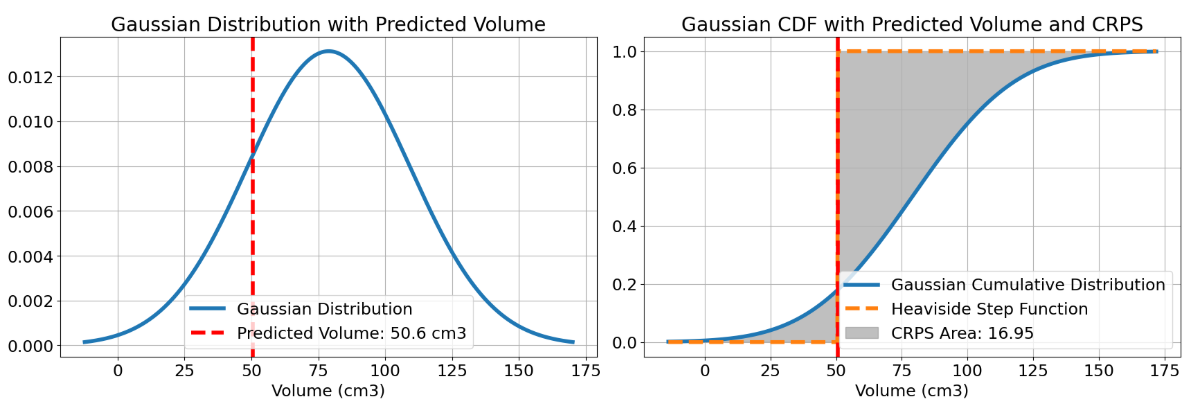
Figure 3 - Visual example of a CRPS calculation.
In conclusion, by using CRPS, we will assess the accuracy of the probabilistic volume prediction relative to the ground truth volume probabilistic distribution.
4. Vascular Invasion
The Vascular Invasion (VI) analysis will be performed for the following five vascular structures: PORTA, Superior Mesenteric Vein (SMV), Superior Mesenteric Artery (SMA), CELIAC TRUNK, and AORTA.
The VI will be computed separately for each structure, with individual rankings produced for each one.
Given the complexity of these anatomical structures, the VI for each vessel will be defined by the most restrictive value observed across all slices in the axial, sagittal, and coronal planes. This involves iterating through every slice in each plane, identifying the vessel boundaries, and determining the proportion of the vessel’s edge that lies within the PDAC. See Figure 4 for reference.
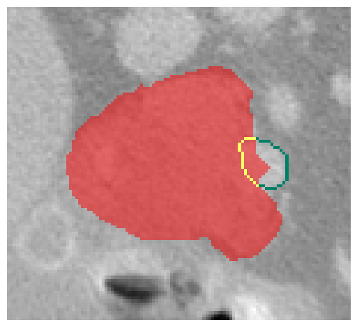
Figure 4 - Visual example of a VI calculation. PDAC (red), part of the vascular structure without invasion (green) and part of the vascular structure invaded (yellow).
To evaluate the quality of the prediction and whether it invades or not a vascular structure, the following process will be used:
- For each vessel, a ground truth (GT) distribution will be generated by computing the VI for each GT annotation. The mean and standard deviation of these values will define a Gaussian distribution.
- For the prediction, the probability map will be thresholded at six levels to produce a set of VI values. These will also form a Gaussian distribution.
- This results in a distribution per vessel and plane for both the GT and the prediction. The Wasserstein distance between these distributions will be computed, with the final metric for each vessel corresponding to the most restrictive distance across all planes.
⚠️ To ensure robust evaluation, the predicted and ground truth distributions are sanitized before computing Wasserstein distances. This involves replacing any NaN or infinite values with zero, clipping negative values (which are invalid in probability distributions) to zero, and normalizing the distributions so that their values sum to 1. These steps ensure numerical stability and fair comparisons, even when inputs are sparse, corrupted, or empty.
The Wasserstein distance is sensitive to: shifts in location (differences in where involvement occurs spatially), and differences in shape or spread of the distributions (how involvement is distributed across slices or planes).
Fair fallback rules are applied when one or both distributions are effectively empty (i.e., sum to zero). These rules preserve absolute magnitude information for meaningful disagreement scoring:
✅ Both GT and prediction are empty → considered a perfect match: score = 0.0
❌ Only one is empty (GT or prediction)
→ If the non-empty distribution is degenerate (zero standard deviation), score = absolute difference between its mean and zero
→ Otherwise, score = maximum penalty (e.g., 360) reflecting maximal disagreement
Final Ranking
The final ranking will be defined by the mean rank of the different rankings.